There are many different techniques available in cycles analysis and this is a short guide to the main ones and when they are appropriate.

Fourier Analysis is the standard method for converting any time series into the sum of a series of sine waves of different frqeuencies. It is important to understand that any series can be exactly constructed from sine waves and so it does not prove that real cycles exist. However if a graph is made of the amplitude versus frequency of the components then real cycles will stand out as having much higher amplitudes, possibly on several adjacent frequencies. There are methods to interpolate the frequency and find the best estimate for each cycle that is considered real.

It is desirable to have certain characteristics in data before it is analysed for cycles. One of these is that the fluctuations are of similarly meaningful amplitude of the time period. When a Stock Market Index of 200 years is constructed we find that, partly due to inflation, the index has grown in a compound manner. For data of this type taking logarithms before looking for cycles is highly desirable. This is true of all measurements made in currencies and with population bases, especially if they are long term series. If the result of taking logs is to make the short and medium term variations more consistent in amplitude over the whole series then it is probably a good idea.

Another useful prepatory function is to take differences of adjacent data points. This is applicable for price data also, as we then create a rate of price change series which is generally more interesting. When it comes to making predictions then we want to know whether it will go up or down and by how much. When this technique is used the spectrum has the same peaks but the shorter term ones are emphasised at the expense of the longer ones.

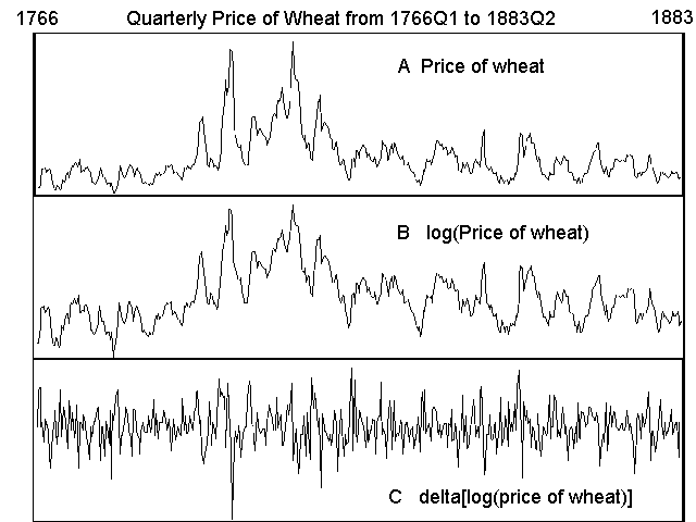
Example 1 shows the Price of Wheat over a period of more than 100 years. Because this was last century, not this century, there is little inflation overall although the price varied considerably. In A the raw data shows wider variations near the middle of the period when the price was higher. This is a case where taking logs is recommended and in B we see that this results in more even short term fluctuations. Finally, in C the result of taking differences between adjacent values is shown. The cycle of about 5.5 years is still visible, but the shorter term fluctuations are now stronger and the longer term ones have all but vanished.

Having prepared our data we are finally ready to do a Fourier analysis. In general cycles of more than 2 time intervals can be detected but there is a danger of "aliasing" for cycles at the very short end. Aliasing means that the wrong period is determined because the measurement interval is too short for the cycle.

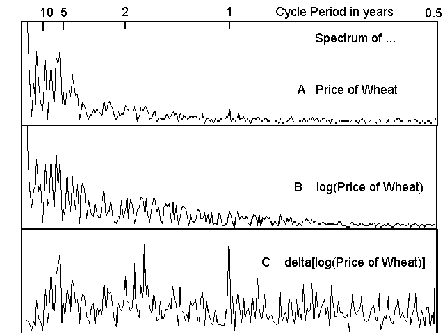
Example 2 shows the spectra obtained from the above cases A, B and C. With quarterly prices it is not possible to detect cycles of less than 1/2 a year. A cycle of exactly one year is present and it is especially easy to see in C. Of course a 1 year cycle is just the seasons and we would expect the price of wheat to vary with the seasons as it is a seasonal crop and requires storage costs to be available at other times.

There are the same set of cycles which are present in all three graphs in the 5 to 20 year range. The strongest of these is about 5.5 years and is clearly visible in the original data without much imagination. In B this peak is split into 2 while in A and C it is almost split. This indicates that the cycle is modulated on a long term basis. The modulation may be just a result of changing circumstances and have no ongoing basis.

The accurate periods found in C are 1.001, 1.697, 4.20, 4.75, 5.54, 7.3, 9.1, 14.3 years. The strongest ones are the 1 year, the 1.697 year and the 5.54 year cycles. These 3 cycles are almost certainly real and C has correlation coeficients of .225, .198 and .187 respectively with sine waves of the stated periods. The seasonal one would not be disputed.

The period 5.54 years is exactly half of the average sunspot cycle period. There has been debate about the role of sunspots in affecting the weather and life on earth. However in recent years improved data and methods have shown that there is no doubt that the earth is affected by variations in the sun. But why half? Well, if the sunspot cycle does affect the weather and in turn how well wheat grows then we would expect the variations to be go beyond optimum condition in two directions (be it too hot and too cold or too wet and too dry) and therefore in one sunspot cycle there would be two cycles in wheat growth.

The 1.697 year period is also interesting. There is a weak cycle at 3.39 years which is exactly double that period. The 3.39 year (40.68 month) cycle is also the dominant cycle in the US stock market and commonly called the 40 month cycle and is, according to Dewey, the most commonly reported cycle of all. This finding of cycles that are exactly half as long as others is a very common occurence. They are called harmonics. Finding cycles of the same length in different series is also common.

You may wonder why the periods are back to front and all bunched up at one end. This is because Fourier analysis measures frequency not period and we calculate the period as 1/frequency. On a frequency basis it is uniformly spread.