DESCRIPTION
1-B EXPLORATORY DATA ANALYSIS
In this exercise, students are required to identify and analyze a digital audio signal with some added noise. As you are likely to be aware, when someone records data, the signal of interest is often corrupted by noise. Because of this, the objective of this exercise is to identify these unknown noise signals and eliminate them using non-real-time digital filtering techniques in MATLAB.
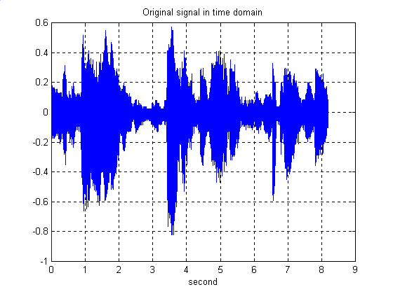
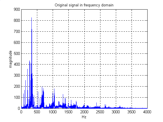
In this part of the experiment, students are required to qualitatively identify the differences between the original signal and the noisy signal in both time and frequency domains. Follow below procedures:
1. Collect your set of signals based on the last digit of your student ID.
2. Use MATLAB to analyze these signals. Yours analysis of these signals should focus on both the time and spectral domains.
Here is an example of MATLAB codes to perform the time and frequency domain analysis of the original signal in MATLAB.
%read sound files
%signal is the vector holding the original
samples & freq refers to the sampling frequency
[signal,freq]= wavread('orig1.wav');
n = length (signal);
%Length of the original signal
%plot original signal in time domain;
figure;
plot ((1:n)/freq,signal);
title('Original signal in time domain');
xlabel ('second');
grid;
%plot a original signal in frequency domain
figure;
signal0=signal -mean (signal); %remove
DC component
fsignal=fft(signal0);
%use fast fourier transform to transform the original
signal into frequency domain.
plot ((1:n/2)/n*freq, abs(fsignal(1:n/2)));
title('Original signal in frequency domain');
xlabel ('Hz');
ylabel('Magnitude');
grid;
figure;
plot((1:n/2)/n*freq, unwrap(angle(fsignal(1:n/2))));
title ('Original signal in frequency domain');
xlabel ('Hz');
ylabel ('Phase');
grid;
3. Understand the example codes in Section (2),
based on the above codes, create a MATLAB program that can perform the
time and frequency domains analysis for the given original and noisy .wav
files. Show your plot using this new MATLAB program on both time and frequency
domain of the original and noisy signals to the instructor, and identify
the noise of the noisy signals.
1-C: DESIGN AND IMPLEMENTATION OF LOWPASS FIR FILTERS
1. There are four specification of the lowpass FIR filter to be observed, as shown in Figure 1.1.
Stopband edge frequency, fs
-Lowpass filter will blocked signals with frequency above fs.
Passband edge frequency, fp
-Lowpass filter will preserved signals with frequencied below fp as
it is.
Pass band gain, Gp
-Gain in dB for passband frequencies.
Stopband attenuation, Gs
-Attenuation gain in dB for stopband frequencies.
Note that, practically, a transition band frequency (fs-fp) exists for any practical lowpass filter.
2. The noisy signal is, in fact, a combination of
many signals with different frequencies. In using fir1 MATLAB command,
we need to determine the cutoff frequency, fc. The argument wn, in fir
function representing normalized cutoff frequency, and usually it is given
by:
![]() (2)
(2)
Where fT is the sampling frequency.
Refer to plots and results in Section 1-B, determine fp and fs, and
then fc and Wn.
3. Argument N in the fir1 function representing the length (number of impulses) of the lowpass filter. Longer N gives better filtering effects (better passband and attenuation), however, it needs more computations. For this experiment, you should achieve a passband gain |Gp| < 3dB and stopbacd sttentuation |Gs| > 20dB. Determine the minimum filter length N that can be used to obtain a lowpass FIR filter that fulfills the passband and stopband specfications.
4. Design the FIR using fir1 MATLAB function. Plot the designed
frequency responses (Magnitude and Phase) to see whether the specifications
are met especially check the passband and stopband edge frequencies, they
may not the same as the input to the function. Save the filter coefficients
into a file if the filter satisfies the specification, otherwise redesigns
the filter with different set of parameters. Plot the impulse response
of the filter, i.e. its coefficients using stem function.
5. Remove the noise of the noisy signal using the designed
filter by the filter()MATLAB function. For example, if the noisy signal
is stored in the vector x and the designed FIR filter coefficients are
stored on the vector h, then we can obtain the filtered signal by
Y=filter(h,1,x)
6. Evaluate the effectiveness of the designed filter by
computing the MSE (mean squared error) and SNR (signal to noise ratio)
between the original signal and the filtered noisy signal. The MSE and
SNR are defined as:
 (3) & (4)
Where s(n) is the original signal sample, y(n) is the filtered signal
sample, and M is the total number of samples. Write MATLAB codes to compute
the MSE and SNR. What is the SNR that you obtained for the Filtered signal?
What is the SNR for the noisy signal before filtering?
Plot the original and filtered signal
on the same figure for both time and frequency domains. How does the filtered
signal sound? Students are reminded that the filtered signal is required
to save in .wav format and available in your personal web site for evaluating
the quality of your reconstructed signal.
7. In DSP chip, a coefficient is usually represented
using a finite number of bits, e.g. 8-bit DSP chip. Write a MATLAB program
to quantize the coefficients of the filter into 4-bit, 8-bit, 12-bit and
16-bit. The quantization program basically, perform the following computation:
![]() (5)
(5)
Where ![]() is the floor operator,
N is the number of bits, bk and Bk are the unquantized and quantized filter
coefficients, respectively.
is the floor operator,
N is the number of bits, bk and Bk are the unquantized and quantized filter
coefficients, respectively.
To experience the coefficient quantization effect, measure the frequency
response of the filters with quantized coefficients, and find out the smallest
number of bits required for the FIR filter that can satisfy your specifications
without redesign the filter.
8. Evaluate the effectiveness of the design
with quantized by computing the MSE and SNR between the original signal
and the filtered version of the noisy signal. Plot the original and filtered
signal on the same figure for both time and frequency domains. How does
the filtered version sound? What can you comment on the effects of filter
coefficient quantization to filters performance.
RESULTS
To achieve the best filtering effect, the specification values below are the most suitable:
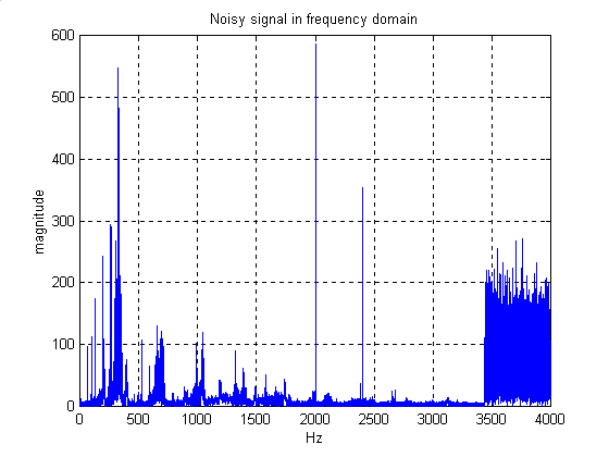
1. Stopband edge frequency, fs = 2000 Hz
2. Passband edge frequency, fp = 1500 Hz
3. Cutoff Frequency, fc
= (fs + fp)/2 = (2000 + 1500)/2 = 1750 Hz
4. Passband gain, |Gp|
= 1dB
5. Stopband attenuation, |Gs|
= 50dB
List of figures:
Original Signal In Time Domain
Original Signal In Frequency Domain ( Magnitude Response, Phase
Response)
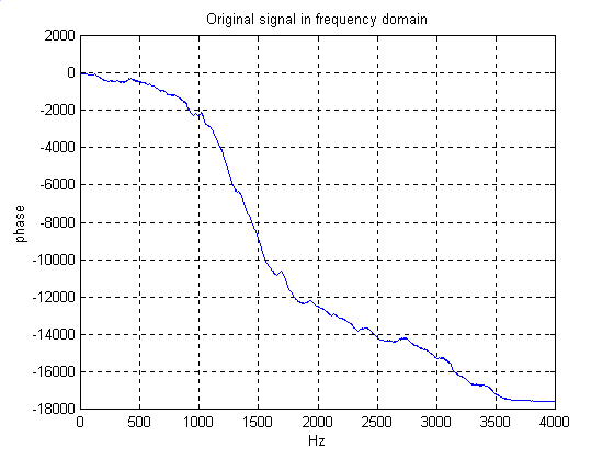
Noisy Signal In Time Domain
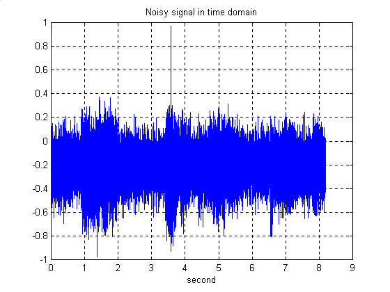
Noisy Signal In Frequency Domain ( Magnitude Response, Phase Response)

Filtered Signal In Time Domain

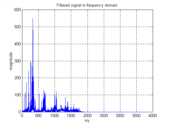
Filtered Signal In Frequency Domain ( Magnitude Response, Phase
Response)
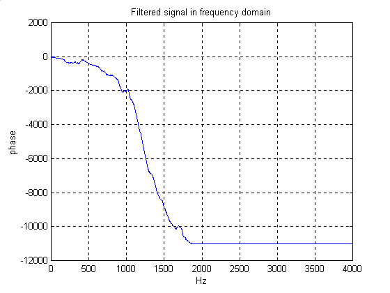
Frequency Response ( Magnitude and Phase )

Sounds:
|
( noisy1.wav ) Original Signal |
( orig1.wav ) Filtered Signal |
( fir1.wav ) |
Quantization:
Figures of 4-bit, 8-bit, 12-bit, 16-bit Quantization.
MSE between the noisy signal and the original signal
= 0.0573
MSE beween the filtered signal to the original signal
= 0.0747
SNR for the noisy signal to the original signal (before filtering)
= -5.3796
SNR for the filtered signal to the original signal
= -6.5317
Observation and Elaboration
In this experiment, we have to design a digital FIR low-pass filter according to a special specification. We obtain these specifications, for example in this particular experiment, from the graphs that has been produced. We have some noise in the signal in which our objective is to remove it by implementing the FIR low-pass filter designed.
After we filter out the noisy signal, we should have cut-off the noisy
part of the signal at certain range of frequency.
In calculating the normalized cutoff frequency, we can use the following
expressions:
Wn = 2fc/ft
= ( fp + fs )/ ft
From what we can see, the higher values of SNR means that the signal
has less noise which indicates that it has been filtered.
M-Files Scripts
| FIR Filter Scripts |