A dynamical system is a set of possible states or conditions, together with some rule that determines the immediate state, in terms of the past states.
This is a very similar interpretation to the definition of function (except in this case we have a system of functions). For example, one can think of the simple model:

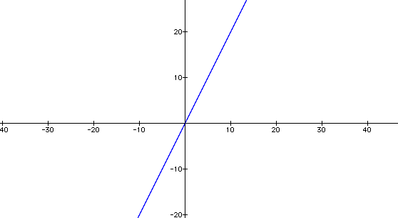
With this function we can find our new condition xn by taking any preceding condition and multiplying it by 2. This rule particularly is termed deterministic, because we can uniquely determine the present state from thee past states. In a deterministic dynamical system there is no room for randomness. A random process is also called a stochastic process. This type of process is not deterministic.
Two types of dynamical systems to bring note of are Discrete Time Dynamical Systems (DTDS) and Continuous Time Dynamical Systems (CTDS). DTDS are those which are taken at different times and the new result of the system is an output based upon the past values. CTDS can be viewed as DTDS whose time differentials are getting infinitly small. The rules which govern CTDS are differential equations.
In the above example we are following the rule f(x)=2x, or alternatively written to show present from past states xn=f(xn-1)=2xn-1 [Note that this type of growth is called exponential growth]. Composition of functions is essential to our understanding in this area.
A functional composition is when we arrive at some functional value, and then plug that value back into the function to achieve a new value. For example:
f(x)=2x is our function. Start at x=2 then f (2)=2 (2)=4
Now compose this with (f) again,
f(x)=2x is our function. Start at x=4 then f (4)=f [f (2)]=2 (4)=8.
Notice the way that these functions are written! In general we define a f^k(x) to be the final result of applying the rule f, to the initial condition k times.
One key feature which we want to investigate is the behaviour of a system. Sometimes we will find patterns which are very simplistic. At other times, overtly chaotic (ha!).
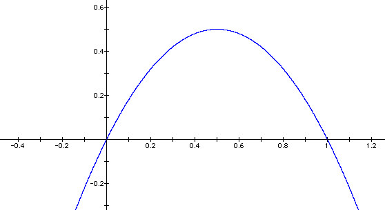
Let us look now at a more interesting model: t(x)=2x(1-x)
We allow this model to represent population population growth with resource limitations. Say x is measured in millions and we have an intitial population of 10,000 which corresponds to x=.01. Notice the two "separate parts" of this function, 2x and (1-x). When x is small (very close to zero) then (1-x) is very close to 1, which makes this function similar to the above f(x)=2x. But when x is large then this example illistrates a non-linear effect.
Ā
We use excel to investigate the behaviour of f(x)=2x and g(x)=2x(1-x) under reflexive functional composition.
| g(x)=2x(1-x) |
|
|
|
|
|
|
|
|
|
|
|
|
|
|
|
|
|
|
|
|
|
|
|
|
|
|
|
|
|
|
|
|
|
|
|
|
|
|
|
|
|
|
|
|
|
|
|
|
|
|
|
|
|
|
|
|
|
|
|
|
|
|
|
Wow! What happend? It seems that our logistic growth model of g(x)=2x(1-x) has reached a limit. Or has been attracted to the fixed value (.5). Let's try other initial starting values and see what happens:
| g(x)=2x(1-x) |
|
|
|
|
|
|
|
|
|
| # of Comps |
|
|
|
|
|
|
|
|
|
|
|
|
|
|
|
|
|
|
|
|
|
0.376062054445875 |
|
|
|
|
0.469278771303646 | 0.499999997847664 |
|
|
|
0.498112412214773 |
|
|
|
|
0.499992874024706 |
|
|
|
|
0.499999999898441 |
|
|
|
|
|
|
|
|
|
|
|
|
|
|
|
|
|
|
|
|
|
|
|
|
|
|
|
|
|
|
|
|
|
|
|
|
|
|
|
|
|
|
|
|
|
|
|
|
|
|
|
|
|
|
|
|
Let's overlay the graph with the graph of f(x)=x
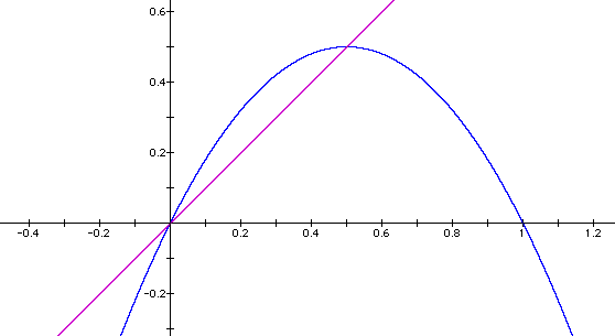
We have the following:
A function whose domain is the same as it's range space shall be called a map. Let x be a point (x0 is the initial condition/ value) under a mapping f. The orbit of x under f is the set of points O={x, f(x), f^2(x),... } remember functional compositions ? A point p is a fixed point of the map f if f(p)=p (as in the above graph when f(x)=x).
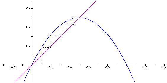
We know from the above definition that whenever a graph intersects the line f(x)=x, this will result in a fixed point. Now the idea behind a "cob-web" plot is to watch the path, or orbit of a given initial condition. This is accomplished at follows:
Start with whatever initial condition one desires (say x=.05) then compute f(.05) and draw a vertical line from the IV in our domain to the point of intersection with the function. Next draw a horizontal line from this intersection point to the line f(x)=x. Now compose the function again, taking f(f(.05)) from the intersection with f(x)=x. This gives us a vertical line. Repeat this iterative procedure a few times. Notice how the path of our intial value converges to the same value as in out spreadsheets.
|
|
|
|
|
|
|
|
|
|
|
|
|
|
|
|
|
|
|
|
|
|
|
|
|
|
|
|
|
|
|
|
|
|
|
|
|
|
|
|
|
|
|
|
|
|
|
|
|
|
|
|
|
|
|
|
|
|
|
|
|
|
|
|
|
|
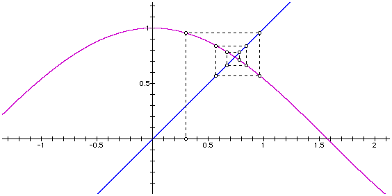
Now we have a pretty good idea of what a fixed point is. Let's explore this concept more in depth. In the graph of f(x)=2x(1-x) we have two fixed points in the shown domain and range (namely at 0 and .5).

It seems that .5 is attracting the orbit of our point starting at .1, where as zero is not. From here we define two types of fixed points, stable and unstable fixed points. Stable fixed points have the property that points which are near to the stable fixed point, under a particular dynamical system (rules) will move towards this point. Unstable fixed points have the property that points near to the unstable fixed point will move away.
Why is stability important?
Well think of the universal laws of attraction and repulsion. In a given instance we may want to know when a given thing is going to attract somthing, or repel it. Real life systems may be very sensitive, and small perturbations or disturbances may cause unforseen fluctuations
An important question arrises when one asks oneself,"What does near mean?" When approaching this question we make use of the concept of derivative. In this case we use the derivative to measure to expansion or contraction factor of a given function. By expansion we mean a measure of the amount that a point moves away from a fixed point, whereas by contraction we mean a measure of the amount of drawing towards a fixed point. In other words given some point p and a fixed point P* (.1 and 0 in the above case), after taking the image of p and P* (0, .1) under f the distance separating the points is approximately altered by a factor of f'(0) [remember the notion of derivative as the rate of change of a function?].
Let us have the precise mathematical notion of this from analysis:
A smooth map is a continuous and infinitely differential function.
First we define some small neighborhood, or ball of radius epsilon e about a point p, Ne(p).
(let R=R^1 or the real axis, and let el="element of", and let oo be (hehe) infinity, and ~= is "not equal to")
Ne(p) = {x el R: | x - p | < e}
Now given f a mapping on R, and p el R such that f(p)=p.
Then if there exists an e > 0 such that for all x el Ne(p), limj-->oo f ^ j(x)=p, then p is an attracting fixed point or a sink. If there exists an e > 0 such that for all x el Ne(p), limj-->oo f^ j (x)~=p, that is as we iterate functional compositions and all points in an epsilon ball eventually get pushed away from p, then p is a source.
We have the following theorem concerning sinks and sources relating the derivative.
Theorem I: Let f be a smooth map on R, and p is a fixed point of f, then
a) If |f '(p)| < 1, then p is a sink
b) If |f '(p)| > 1, then p is a source
Extended result |f^k(x) - p| <=(a)^k |x - p| for a<1, f^k(x) converges exponentially to p as k-->oo
Let us first think about this before attempting a proof. This is saying that if the absolute value of the derivative about p is less than one then p will be a sink, and if the absolute value of the derivative is greater than one about p, then p is a source. Well the derivative is the rate of change of the function and if this rate of change is a fraction (less than one) then the successive functional compositions will yield smaller and smaller functional outputs. Think of this as multiplying a number by a unit fraction. What happens to the number? --> it gets smaller and smaller (ie 8*.5 =4 then 4*.5 =2 then 2*.5 =1 etc...).
The proof of part a) and the extended result is given by book A (see reference pg 10). For part b) the proof is as follows:
Let a be any number between |f'(p)| and 1; that is |f'(p)|> a >1.
Now we have (by definition) limx->p |f(x) - f(p)| / |x - p| = |f'(p)|.
There is some ball of radius positive epsilon [Ne(p)] about p, so that
|f(x) - f(p)|/ |x - p| > a for all x el Ne(p).
Why is this so? Well because of a being between 1 and |f'(p)| so there must be some values about p which are greater than a. this implies that if x el Ne(p) then f(x) el Ne(p) and successive derivatives will get mapped outside.
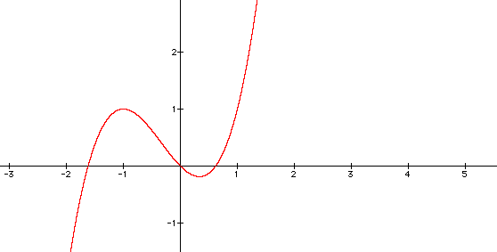
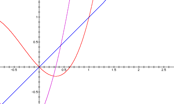
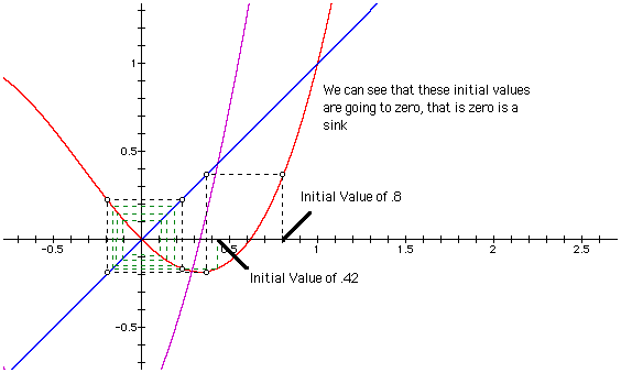
In the given domain and range we can see that there are two fixed points and the derivative is less than 1. By the above theorem we should have an attracting point at zero. Lets try a cobweb plot.
| f(x)=x^3 +x^2-x |
| Iterations |
|
|
|
|
|
|
|
|
|
|
|
|
-0.148750319519381 | 0.212236756685651 |
|
|
0.167585629694982 | -0.157632229756325 |
|
|
-0.134794053510147 | 0.17856331660226 |
|
|
0.150514358327259 | -0.140984992565961 |
|
|
-0.124449947887402 | 0.158059434687907 |
|
|
0.138010282816782 | -0.129127884936793 |
|
|
-0.116334785131949 | 0.143648815874038 |
|
|
0.128294117715699 | -0.120049642798759 |
|
|
-0.109723095357836 | 0.132731414078653 |
|
|
0.120441279369344 | -0.112775373080577 |
|
|
-0.104188044136641 | 0.124059348543768 |
|
|
0.113912215982358 | -0.106759263642551 |
|
|
-0.0994580989208396 | 0.11694001099844 |
|
|
|
-0.101665894131531 |
|
|
|
0.110951034152977 |
|
|
|
-0.0972750802996637 |
|
|
-0.0917362280795904 | 0.105817061814807 |
|
|
0.0993797541339434 | -0.0934349510878485 |
| 1350 | 0.0136349497416733 | -0.01346108252737 |
| 1351 | -0.0134465029884234 | 0.0136398441120257 |
| 1352 | 0.0136248801897771 | -0.013451261135089 |
| 1353 | -0.0134367135428 | 0.0136297637380967 |
| 1354 | 0.0136148328785456 | -0.0134414612710671 |
| 1355 | -0.0134269455087874 | 0.0136197056446347 |
| 1356 | 0.0136048077262695 | -0.0134316828566693 |
| 1357 | -0.0134171988083464 | 0.0136096697497255 |
| 1358 | 0.0135948046516588 | -0.0134219258136623 |
| 1359 | -0.0134074733638358 | 0.0135996559718761 |
| 1360 | 0.0135848235738405 | -0.0134121900642122 |
| 1361 | -0.0133977690980098 | 0.0135896642300115 |
| 1362 | 0.0135748644123556 | -0.0134024755308817 |
| 1363 | -0.0133880859340151 | 0.0135796944434722 |
We can see that this limit will goto zero.
Let's look at the following and close this out.
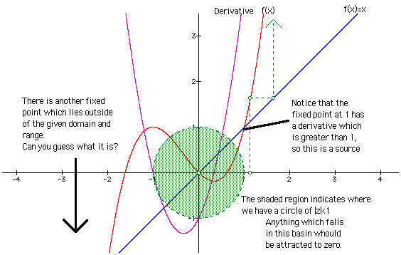
In the beginning of the next essay we shall formalize the idea of a basin of attraction and present material on logistic maps and other interesting things.