Naive Bayes Models for Classification

A Tutorial

Bill Majoros
July 22, 1999

Introduction

The Naive Bayes Model is a simple and well-known method for performing supervised learning of a classification problem. It is based on a simple result from elementary statistics known as Bayes' Theorem. The method is relatively easy to code in software, and occasionally performs quite well, though it has a reputation for being inferior to more sophisticated techniques.

Statistical Background -- Bayes' Theorem

Assume a sample space, S, which is partitioned into n subspaces, Xi, for integer i in [1,n]. Suppose that an event, Y, occurs, where Y is a set of sample points in S. That is, we know only that the sample point drawn from S was one of the points in Y. We do not know which partition (i.e., which Xi) contained the point.

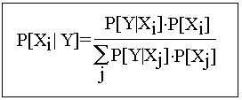
Then the probability of the point occurring in Xi is given by the following:

That is, the conditional probability of Xi given Y is equal to the value of the expression on the right. This is known as Bayes' Theorem, and it can be easily derived through the use of simple statistical identities (in particular, the repeated application of the so-called Multiplication rule: P[A & B]=P[A|B]*P[B]).

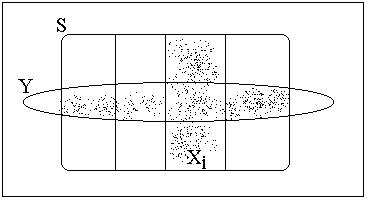
To develop an intuitive understanding of Bayes' Theorem, consider the sample space shown below:

Imagine that a sample point has been drawn from S, and we know only that the point lies in Y. Then the probability that that point also happens to lie in Xi can be assessed by computing the proportion of points in Y that actually lie in the intersection between Y and Xi. In Bayes' Theorem, the numerator counts the points in the intersection, and the denominator sums all the points in Y.

The relevance of Bayes' Theorem to the problem of classification will be made clear shortly.

Classification and Supervised Learning

In a classification task, one is given an object having some set of attributes and is expected to correctly classify the object into one of several predefined categories. The attributes of the incoming objects vary, and one hopes that the classification can be done based on the actual values of these attributes.

In a supervised learning scenario, the classifier is provided with a set of training examples prior to performing the real classification task. Each training example consists of an object to be classified, as well as the correct category to which it should be assigned. Thus, we begin with a learning phase, during which the classifier analyzes the training examples and builds a model to store any knowledge which was learned about the problem space. This model is later applied to help the classifier perform the real classification task.

In this case, we are concerned with classifiers that build a Naive Bayes Model to perform classification.

The Naive Bayes Model

If we consider Y to be an object to be classified, then Bayes' Theorem can be read as a formula for the probability that Y belongs in category Xi. Assuming that the conditional probabilities for different Xi differ, it is reasonable to simply assign Y to the Xi having the highest conditional probability (i.e., conditional upon the attribute values of Y).

Since the denominator in Bayes' Theorem is independent of i (and is always nonnegative), the numerator of the most likely Xi will also have the greatest magnitude. Thus, to perform classification, we need only compute the numerator in Bayes' Theorem for each Xi and then pick the Xi giving the largest value.

The problem has now been reduced to computing P[Y|Xi]*P[Xi].

P[Xi] can be trivially estimated by counting the training examples that fall into Xi and dividing by the size of the training set.

P[Y|Xi] is less trivial, and it is the computation of this term that warrants use of the word naive in the phrase Naive Bayes Model. The model is naive in the sense that it assumes (often unjustifiably) that the attribute values of object Y are independent.

Under this assumption, we can compute P[Y|Xi] by simply multiplying together the conditional probabilities of the attribute values of Y. For example, if Y has attributes color=blue and texture=smooth, we can (presumably) estimate P[Y|Xi] by computing P[blue|Xi]*P[smooth|Xi].

These conditional probabilities can be estimated by simply observing the distribution of attribute values within Xi in the training set. Thus, if half of the training examples in Xi are blue and one-third are smooth, and if Xi contained 75% of the training set, then we would assess the probability of Y belonging to Xi as 1/2 * 1/3 * 3/4 = 1/24, or approximately 4.2%. If this turned out to be the highest probability, we would assign Y to Xi.

Implementing the Method in Software

With the proper data structures, this method is relatively easy to code in software. The P[Xi] values can be precomputed by tabulating instances of training examples that fall into each category. The P[Y|Xi] requires a three-dimensional data structure to tabulate the occurrences of attribute values in each category.

Once these data structures have been computed, it is a simple matter to classify a new test case; one need only perform a series of table look-ups and multiplications in order to compute the numerators in Bayes' Theorem, and then simply select the Xi having the greatest such value.

Conclusion

The Naive Bayes Model is clearly an easy approach to supervised learning of classification tasks. On test problems, one will often find that it performs less well than other methods, such as backpropagation neural networks, but occasionally, it will perform better than one or more competing techniques.

The method performs best when attribute values approach independence. For problems where attributes have many complex interactions, there is less reason for optimism. However, the Naive Bayes Model is a good candidate for a first attempt at learning a new classification task.