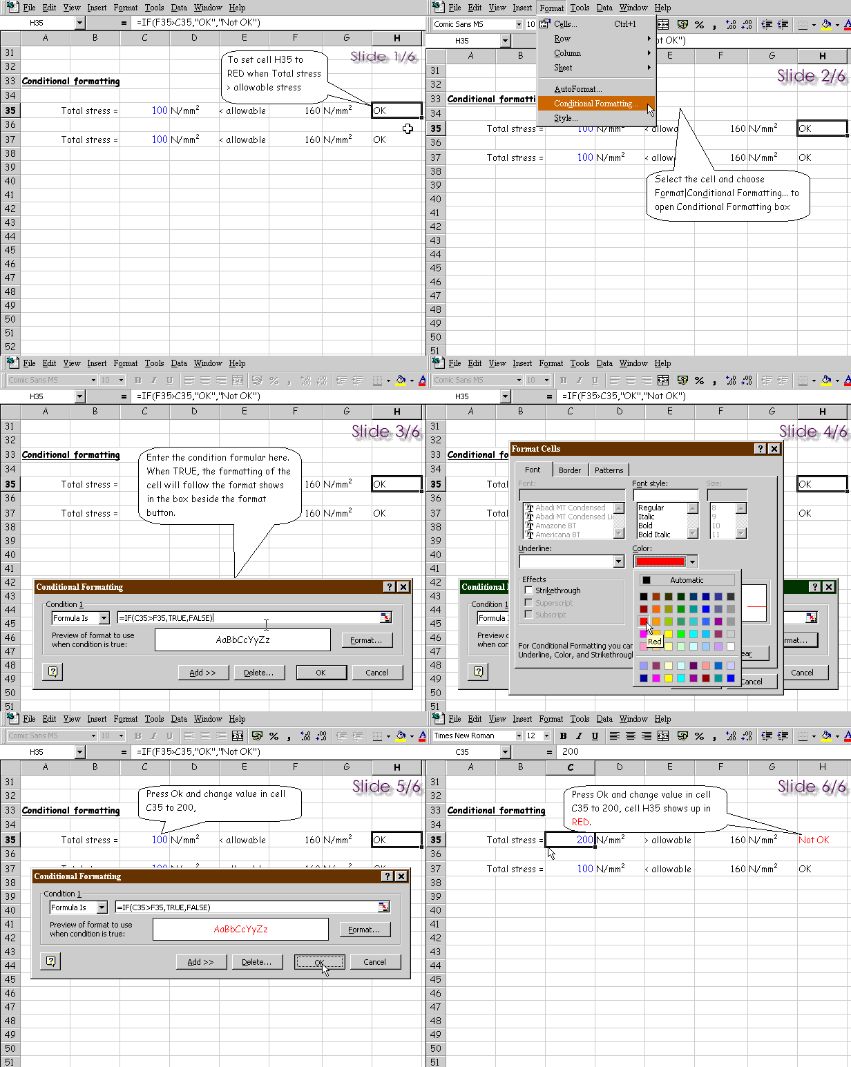
To apply conditional formatting to a cell, follow the step below.

1. Select the cells you want to format.
2. On the Format menu, click Conditional Formatting.
3. To use values in the selected cells as the formatting criteria, click Cell Value Is, select the comparison phrase and then type a value in the appropriate box. You can enter a constant value or a formula; you must include an equal sign (=) before the formula.
4. To evaluate data or a condition other than the values in the selected cells, use a formula as the formatting criteria. Click Formula Is in the box on the left, and then enter the formula in the box on the right. The formula must evaluate to a logical value of TRUE or FALSE.
5. Click Format.
6. Select the font style, font colour, underlining, borders, shading, or patterns you want to apply.
7. Excel applies the selected formats only if the cell value meets the condition or if the formula returns a value of TRUE.
   
   The slide show demonstrate the steps to apply conditional format to a cell.

.

The above sample is available for downloading.

Thanks to for hosting this page. Get your own free home page too.