Beginners Guide To Microsoft Excel

What is a spreadsheet ?

A spreadsheet is the computer equivalent of a paper ledger sheet. It consists of a grid made from columns and rows. It is an environment that can make number manipulation easy and somewhat painless.

The math that goes on behind the scenes on the paper ledger can be overwhelming. If you change the loan amount, you will have to start the math all over again (from scratch). But let's take a closer look at the computer version.

 Looking at our previous example it seems pretty evenly matched. Right? WRONG! The nice thing about using a computer and spreadsheet is that you can experiment with numbers without having to RE-DO all the calculations. Lets change the interest rate and then the number of months. Let the COMPUTER do the calculations! Once we have the formulas setup, we can change the variables that are called from the formula and watch the changes.

Do that on paper and you better get your calculator back out, and get an Eraser and hope you punched all the right keys and in the right order. Spreadsheets are instantly updated if one of the entries is changed.
NO erasers! NO new formulas! NO calculators!

Spreadsheets can be very valuable tools in business. They are often used to play out a series of what-if scenarios! (much like our car purchase here.)

 What is a spreadsheet made up of ?

So let's get started digging into what makes a spreadsheet work. Spreadsheets are made up of

• columns
• rows
• and their intersections are called cells

In each cell there may be the following types of data

• text
• number data
• formulas

Take a look at the explanations of each of these.
Remember there will be a short quiz later on so if there is something you need to take notes on,
TAKE NOTES ON IT!

In a spreadsheet the COLUMN is defined as the vertical space that is going up and down the window. Letters are used to designate each COLUMN'S location.

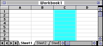
In the above diagram the COLUMN labeled C is highlighted.

In a spreadsheet the ROW is defined as the horizontal space that is going across the window. Numbers are used to designate each ROW'S location.

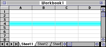
In the above diagram the ROW labeled 4 is highlighted.

In a spreadsheet the CELL is defined as the space where a specified row and column intersect. Each CELL is assigned a name according to its COLUMN letter and ROW number.

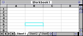
In the above diagram the CELL labeled B6 is highlighted. When referencing a cell, you should put the column first and the row second.

In a spreadsheet there are three basic types of data that can be entered.

• labels - (text with no numerical value)
• constants - (just a number -- constant value)
• formulas* - (a mathematical equation used to calculate)

*ALL formulas MUST begin with an equal sign (=).

 Labels

Labels are text entries. They do not have a value associated with them. We typically use labels to identify what we are talking about.

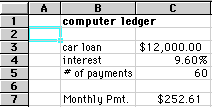In our first example: the labels were

• computer ledger
• car loan
• interest
• # of payments
• Monthly Pmt.

Again, we use labels to help identify what we are talking about. The labels are NOT for the computer but rather for US so we can clarify what we are doing.

 Constants

Constants are entries that have a specific fixed value. If someone asks you how old you are, you would answer with a specific answer. Sure, other people will have different answers, but it is a fixed value for each person.

In our first example: the constants were

• $12,000
• 9.6%
• 60

As you can see from these examples there may be different types of numbers. Sometimes constants are referring to dollars, sometimes referring to percentages, and other times referring to a number of items (in this case 60 months) .These are typed into the computer with just the numbers and are changed to display their type of number by formatting (we will talk about this later).
Again, we use constants to enter FIXED number data.

Formulas 

Formulas are entries that have an equation that calculates the value to display. We DO NOT type in the numbers we are looking for; we type in the equation. This equation will be updated upon the change or entry of any data that is referenced in the equation.

In our first example, the solution was $252.61
This was NOT typed into the keyboard. The formula that was typed into the spreadsheet was:
=PMT(C4/12,C5,-C3)

C4 (annual interest rate) was divided by 12 because there are 12 months in a year. Dividing by 12 will give us the interest rate for the payment period - in this case a payment period of one month.

It is also important to type in the reference to the constants instead of the constants. Had I entered =PMT(.096,60,-12000) my formula would only work for that particular set of data. I could change the months above and the payment would not change. Remember to enter the cell where the data is stored and NOT the data itself.

Formulas are mathematical equations. There is a list of the functions available within Excel under the menu INSERT down to Function.

Formulas OR Functions MUST BEGIN with an equal sign (=).

Again, we use formulas to CALCULATE a value to be displayed.

Constructing Formulas

When we are entering formulas into a spreadsheet we want to make as many references as possible to existing data. If we can reference that information we don't have to type it in again. AND more importantly if that OTHER information changes, we DO-NOT have to change the equations.

If you work for 23 hours and make $5.36 an hour, how much do you make? We can set up this situation using

• three labels
• two constants
• one equation

Let's look at this equation in B4:

• = B1 * B2
• = 23 * 5.36

Both of these equations will produce the same answers, but one is much more useful than the other.
DO YOU KNOW which is BEST and WHY?

It is BEST if we can Reference as much data as possible as opposed to typing data into equations.

In our last example, things were pretty straightforward. We had number of hours worked multiplied by wage per hour and we got our total pay. Once you have a working spreadsheet you can save your work and use it at a later time. If we referenced the actual cells (instead of typing the data into the equation) we could update the entire spreadsheet by just typing in the NEW Hours worked. And -- you're done!

Let's look at the new spreadsheet:

• hours have been changed to 34
• wage is the same
• total pay would now be = 34 * 5.36
• but would still be = B1 * B2

If we had typed in ( = 23 * 5.36 ) the first time and just changed the hours worked, our equation in B4 would still be ( = 23 * 5.36 )

INSTEAD we typed in references to the data that we wanted to use in the equation.
We typed in ( = B1 * B2 ). These are the locations of the data that we want to use in our equation.

It is BEST if we can Reference as much data as possible as opposed to typing data into equations.

Math Function examples

Spreadsheets have many Math functions built into them. Of the most basic operations are the standard multiply, divide, add and subtract. These operations follow the order of operations (just like algebra). Let's look at some examples.

For these following examples lets consider the following data:

Selecting cells is a very important concept of a spreadsheet. We need to know how to reference the data in other parts of the spreadsheet. When entering your selection you may use the keyboard or the mouse.
We can select several cells together if we can specify a starting cell and a stopping cell. This will select ALL the cells within this specified BLOCK of cells.

For this following examples lets consider the following data:

This is just a discussion of selection methods. If we wanted to add the cells in the (To Select) you would type in

=sum(Type In)
or
=sum(Click On)

 The =SUM Function

Probably the most popular function in any spreadsheet is the SUM function. The Sum function takes all of the values in each of the specified cells and totals their values. The syntax is:

• =SUM(first value, second value, etc)

In the first and second spots you can enter any of the following (constant, cell, range of cells).

• Blank cells will return a value of zero to be added to the total.
• Text cells can not be added to a number and will produce an error.

 The =Average Function

There are many functions built into many spreadsheets. One of the first ones that we are going to discuss is the Average function. The average function finds the average of the specified data. (Simplifies adding all of the indicated cells together and dividing by the total number of cells.) The syntax is as follows.

• =Average (first value, second value, etc.)

Text fields and blank entries are not included in the calculations of the Average Function.

 The =MAX Function

The next function we will discuss is Max (which stand for Maximum). This will return the largest (max) value in the selected range of cells.

• Blank entries are not included in the calculations of the Max Function.
• Text entries are not included in the calculations of the Max Function.

 The =MIN Function

The next function we will discuss is Min (which stands for minimum). This will return the smallest (Min) value in the selected range of cells.

• Blank entries are not included in the calculations of the Min Function.
• Text entries are not included in the calculations of the Min Function.

The =Count Function

The next function we will discuss is Count. This will return the number of entries (actually counts each cell that contains number data) in the selected range of cells.

• Blank entries are not counted.
• Text entries are NOT counted.

The =CountA Function 

The next function we will discuss is CountA. This will return the number of entries (actually counts each cell that contains number data OR text data) in the selected range of cells.

• Blank entries are not Counted.
• Text entries ARE Counted.

The =IF Function

The next function we will discuss is IF. The IF function will check the logical condition of a statement and return one value if true and a different value if false. The syntax is

• =IF (condition, value-if-true, value-if-false)

• value returned may be either a number or text
• if value returned is text, it must be in quotes

 The =PMT Function

The PMT function returns the periodic (in this case monthly) payment for an annuity (in this case a loan). This is the PMT function that was used for the car purchase in the first example. There are a few things that we must know in order for this function to work. To calculate the loan we must know a combination of the following

• (rate) interest rate per period
• (nper) number of payments until repaid
• (pv) present value of the loan (amount we are borrowing)
• (fv) future value of the money (for saving or investing)
• (type) enter 0 or 1 to indicate when payments are due.

=PMT(rate, nper, pv, fv, type)

Note that the rate is per period. If we have an annual interest rate of 9% and we are calculating monthly payments, we must divide the annual interest rate by 12 to calculate the monthly interest rate.

 The = SIN, COS, & TAN Functions

Excel has most of the math and trig functions built into it. If you need to use the SIN, COS, TAN functions, they can be typed into any cell. If you wanted to find:

formula format = sin (degree * pi()/180) returns answer in degrees
formula format = sin (degree) returns answer in radians
To calculate trig functions in degrees you must enter them in convert them - otherwise excel will calculate them in radians.

You can type in either an actual number for the REF or you can also type in a reference from the excel spreadsheet (like A2).

The Help Function Wizard 

In Excel there is a help tool for functions called the Function Wizard.

There are two ways to get the the function wizard. If you look at the Standard Toolbar, the function wizard icon look like like the icon on the right.

The other way to get to the function wizard is to go to the Menu INSERT -- down to FUNCTION.

Either way you get there, at this poing Excel will list all of the functions available. Upon choosing the function, Excel will prompt you for the information it needs to complete the function. Mini descriptions are available for each of the cells. It is often necessary for you to understand the functions in order to be able to figure out these descriptions.

Yeah, I know it would have been nice to know this earlier, but it is important for you to understand how the functions work before you start using the Function Wizard. It is faster to type the basic function in from the keyboard as opposed to going through the steps of this tool.

Well, that is all of the functions we are going to cover.
On to the next phase.

 Repeating the same functions elsewhere

Sometimes when we enter a formula, we need to repeat the same formula for many different cells. In the spreadsheet we can use the copy and paste command. The cell locations in the formula are pasted relative to the position we CUT them from.

Fill Down

If you have a lot of duplicate formulas you can also perform what is referred to as a FILL DOWN. (discussed next).

Often we have several cells that need the same formula (in relationship) to the location it is to be typed into. There is a short cut that is called Fill Down. There are a number of ways to perform this operation. One of the ways is to

1. select the cell that has the original formula
2. hold the shift key down and click on the last cell (in the series that needs the formula)
3. under the edit menu go down to fill and over to down

Fixed Postion Cells 

Sometimes it is necessary to keep a certain position that is not relative to the new cell location. This is possible by inserting a $ before the Column letter or a $ before the Row number (or both). This is called Absolute Positioning.

We can also fill right. We must select the original cell (and the cells to the right) and select from the Edit menu -- Fill and Right.

Answers would be A1=16, B1=17, C1=19.

 Formatting Cells

Spreadsheets can be pretty dry, so we need some tools to dress them up a little. We can use most of the tricks in our word processor to do the formatting of text. We can use : bold face, italics, underline, change the color, align (left, right, center), font size, font, etc.

We need to select the cell (or group of cells) that we wish to change the formatting and then go from the FORMAT menu -- down to CELLS -- click on FONT. Here is a picture of what you will see there. Notice that you can choose to change the alignment as well as several other options.

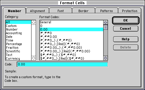
We often need to format the numbers to display the appropriate number of decimals, dollar signs, percentage, red (for negative dollars), etc. It is best to keep numbers describing similar items as uniform as possible.
If we have the number 3.53262624672423, we would probably have to make the column wider and at the least bore most people. We need to set the number of decimal places to what is important. If this was a dollar figure that had calculated tax it should be $3.53.

Here is a screen displaying what you would see if you select a cell (or group of cells) and from the FORMAT menu -- go down to format -- click on number.

A question that everyone (who has ever worked on a spreadsheet) has asked at one time or another is, "Where did all my numbers go?" or same question, "Where did all of those ####### come from and why are they in my spreadsheet?"
The problem is the number trying to be displayed in a particular cell does not have enough width to display properly. To clear up the problem we just need to make the column wider. You can do this many ways.

Here are two ways to change the column width

1. Select the column (or columns) with the problem by clicking on their labels (letters). Then you choose the MENU FORMAT. Go down to COLUMN and over to WIDTH and type in a new number for the column width.
2. Move the arrow to the right side of the column label and click and drag the mouse to the right (to make wider) or left (to make smaller). Let up on the mouse button when the column is wide enough.

Notice the cursor changes to a vertical line with arrows pointing left and right.

In many spreadsheets you can also change the vertical height of a row by moving the lower edge of the row title (number).

Inserting Rows

Likewise, we can also insert rows. With the row label (number) selected you must choose the Row from the Insert menu. Again this will insert a row before the row you have selected.

The formulas will be updated to their corresponding locations.
C3 was = C2+B3
NOW C4=C2+B4

 Charts

Numbers can usually be represented quicker and to a larger audience in a picture format. Excel has a chart program built into its main program. The Chart Wizard will step you through questions that will (basically) draw the chart from the data that you have selected. There are many types of charts. The two most widely used are the bar chart and the pie chart.

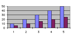The BAR Chart is usually used to display a change (growth or decline) over a time period. You can quickly compare the numbers of two different bar charts to each other.

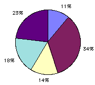The PIE Chart is usually used to look at what makes up a whole Something. If you had a pie chart of where you spent your money you could look at the percentages of dollars spent on food (or any other category).

You can add legends, titles, and change many of the display variables.

• Introduction to Microsoft Office 97
• Introduction to Word Processing
• Complete Microsoft Word 97
• Complete Microsoft Access 97