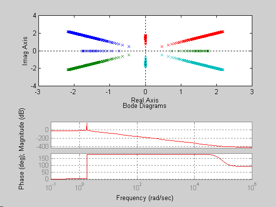
Analyze Open Loop System

The matlab code below was used to analyze the open loop system of the ball balancer.

%Project #1

%Ball Balancer

%Open Loop Analysis

% Set Parameter Values

m=1;

g=9.81;

pn=1;

J=8.81;

%state space matrices

A=[0 1 0 0; 0 0 -g 0; 0 0 0 1; (-m*g)/(m*pn^2+J) 0 0 0];

B=[0; 0; 0; 1/(m*pn^2+J)];

C=[1 0 1 0];

D=[0];

%convert to open loop transfer function

[num,den]=ss2tf(A,B,C,D)

tf(num,den)

k=[-100:0.5:0];

subplot(2,1,1)

rlocus(A,B,C,D,k);

subplot(2,1,2)

bode(num,den);

The transfer function for the system is

Transfer function:

- 1

-------------

s^4 - 9.81

The poles of this system are:

poles =

-1.7698

0 + 1.7698i

0 - 1.7698i

1.7698