State Variable Feedback Controller

The first design I will describe was derived using the State-Variable Feedback (SVFB) technique. The percent overshoot was 4% and settling time was 0.5 sec. The first step is to form the characteristic polynomial

One may solve for alpha by a = 5/ts. So to solve for the natural frequency on must first find the damping ratio, z :

Then follows the natural frequency from:

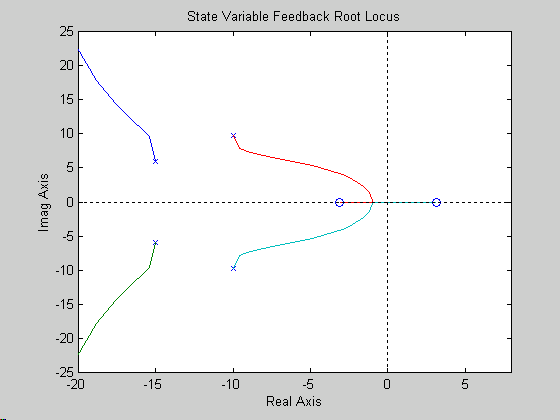
Since the characteristic equation of the open loop transfer function above for the ball balancer is fourth order, two non-dominant poles must be convoluted with the characteristic polynomial to have enough poles for Ackermann’s formula. Using s = -15± j6 as roots the characteristic polynomial becomes:

Now Ackermann’s formula yields the K to simulate the controller:

The vector K is multiplied by x to solve for the input, u:

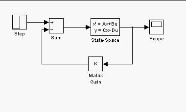
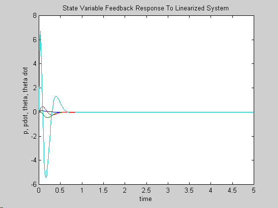
In this project the matlab function acker solves for the vector K given the arguments A, B, and p where A is the system matrix, B is the control input matrix and p is the roots of the characteristic polynomial. The controller stablizes the linear system for a large range of initial values (.01 < x < 10000). Here is the simulink model and matlab code which implements the State-Variable Feedback Design for the ball balancer.

%Project #1

%Ball Balancer

%State Variable Feedback Method

global A;

global B;

global K;

global m; % mass of ball

global g; % gravity

global pn; % nominal point

global J; % inertia of the beam

% Set Parameter Values

m=1;

g=9.81;

pn=1;

J=8.81;

%state space matrices

A=[0 1 0 0; 0 0 -g 0; 0 0 0 1; (-m*g)/(m*pn^2+J) 0 0 0];

B=[0; 0; 0; 1/(m*pn^2+J)];

%C=[1 0 0 0; 0 0 1 0];

C=[1 0 1 0];

D=[0];

[num,den] = ss2tf(A,B,C,D);

[numc,denc] = cloop(num,den);

%Ackerman Method

POV = 4;

ts = 0.5;

alpha = 5/ts;

zeta = 0.716;

wn = alpha/zeta;

deltaD= [1 2*alpha wn^2];

%p = roots(deltaD)

%[Q,R]= deconv(denc,deltaD);

Q = [1 30 261]; % s = -15 +/- j6

deltaC = conv(deltaD,Q);

p = roots(deltaC);

K = acker(A,B,p);

% check the design by computing closed loop poles

Ac = A-B*K;

[numC,denC] = ss2tf(Ac,B,C,D);

% see if denC and deltaC are the same to check design

[numc,denc]=cloop(numC,denC,-1);

t=[0:0.01:5];

y=step(numc,denc,t);

%k=[-100:0.5:0];

%subplot(3,1,1)

%rlocus(Ac,B,C,D);

%subplot(3,1,2)

%plot(t,y);

xo = [.01 .01 .01 .01];

[t,x] = ode23('nonlinear', t, xo);

%subplot(3,2,1)

plot(t,x);

title('State Variable Feedback Response To Linearized System');

xlabel('time');

ylabel('p, pdot, theta, theta dot');

% Project #1 (define nonlinear eqs)

function xdot = nonlinear(t,x);

global A;

global B;

global K;

global m;

global g;

global pn;

global J;

u = -K*x;

%xdot(1) = x(2);

%xdot(2) = x(1)*(x(4)^2) - g*sin(x(3));

%xdot(3) = x(4);

%xdot(4) = (-2*m*x(1)*x(2)*x(3) - m*g*x(1)*cos(x(3) + u))/(m*(x(1)^2) + J);

%xdot = [xdot(1) ; xdot(2); xdot(3) ; xdot(4)];

xdot = A*x+B*u;

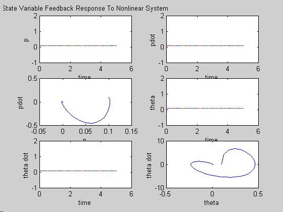
Now I use the nonlinear equations to simulate the controller against a realistic system. The controller stabilizes the system for initial values £ .01.

% Project #1 (define nonlinear eqs)

function xdot = nonlinear(t,x);

global A;

global B;

global K;

global m;

global g;

global pn;

global J;

u = -K*x;

xdot(1) = x(2);

xdot(2) = x(1)*(x(4)^2) - g*sin(x(3));