Digital Controller

The closed loop transfer function from the State Variable Feedback Controller is:

num/den =

-4.263e-014 s^3 - 1.364e-012 s^2 - 2.183e-011 s - 1

---------------------------------------------------

s^4 + 50 s^3 + 1056 s^2 + 1.107e+004 s + 5.091e+004

After a conversion to the z-domain using the c2d function we obtain the z-transform:

-7.97e-007 z^4 - 3.188e-006 z^3 - 4.782e-006 z^2 - 3.188e-006 z - 7.97e-007

---------------------------------------------------------------------------

z^4 - 0.6324 z^3 + 0.3352 z^2 - 0.06315 z + 0.009482

To facillitate the sampling of the continuous system, I used coefficients (a,b,c,d,e,f,g,h,i) to represent the coefficients I obtained from the z-transform.

a = 0.6324; b = -0.3352; c = 0.06315; d = -0.009482; e = -7.97e-007; f = -3.188e-006; g = -4.782e-006;

h = -3.188e-006; i = -7.97e-007;

In order to get the transfer function in to a form to discretize it, one needs to divide through by the highest order and solve for the difference equation in the time-domain:

Y_k = a*y_k-1 + b*y_k-2 + c*y_k-3 + d*y_k-4 + i*u_k + h*u_k-1 + g*u_k-2 + f*u_k-3 + e*u_k-4;

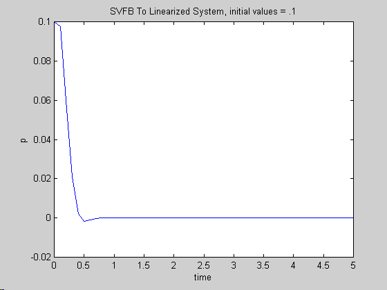
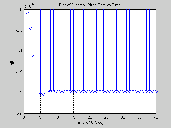
Below is the simulink model and the matlab code which simulates the digital controller, Along with the plots for the continuous system and the digital system versus time.

%Project #1

%Ball Balancer

%State Variable Feedback Method

clear all;

global A;

global B;

global K;

global m; % mass of ball

global g; % gravity

global pn; % nominal point

global J; % inertia of the beam

% Set Parameter Values

m=1;

g=9.81;

pn=1;

J=8.81;

%state space matrices

A=[0 1 0 0; 0 0 -g 0; 0 0 0 1; (-m*g)/(m*pn^2+J) 0 0 0];

B=[0; 0; 0; 1/(m*pn^2+J)];

%C=[1 0 0 0; 0 0 1 0];

C=[1 0 0 0];

D=[0];

[num,den] = ss2tf(A,B,C,D);

[numc,denc] = cloop(num,den);

%Ackerman Method

POV = 4;

ts = 0.5;

alpha = 5/ts;

zeta = 0.716;

wn = alpha/zeta;

deltaD= [1 2*alpha wn^2];

%p = roots(deltaD)

%[Q,R]= deconv(denc,deltaD);

Q = [1 30 261]; % s = -15 +/- j6

deltaC = conv(deltaD,Q);

p = roots(deltaC);

K = acker(A,B,p);

% check the design by computing closed loop poles

Ac = A-B*K;

[numC,denC] = ss2tf(Ac,B,C,D);

% see if denC and deltaC are the same to check design

%Discretization

[numc,denC]=cloop(numC,denC,-1);

%%%%%%%%%%%%%%%%%%%%%%%%%%%%%%%%%%%%%%%%%%%%%%%%%%%%%%%%%%%%%%%%%

% converting the controller using the BLT to a digital controller

T = 0.1;

printsys(numC,denC,'s')

csys = tf(numC, denC)

dsys = c2d(csys, T, 'tustin')

%Transfer function:

%-7.97e-007 z^4 - 3.188e-006 z^3 - 4.782e-006 z^2 - 3.188e-006 z - 7.97e-007

%---------------------------------------------------------------------------

% z^4 - 0.6324 z^3 + 0.3352 z^2 - 0.06315 z + 0.009482

a = 0.6324;

b = -0.3352;

c = 0.06315;

d = -0.009482;

e = -7.97e-007;

f = -3.188e-006;

g = -4.782e-006;

h = -3.188e-006;

i = -7.97e-007;

% Following loop shows discrete sequences for the responses

for k = 1:100

y(k) = 0;

u(k) = 0;

end

for k = 10:100

u(k) = 1;

y(k) = a*y(k-1) + b*y(k-2) + c*y(k-3) + d*y(k-4) + i*u(k) + h*u(k-1) + g*u(k-2) + f*u(k-3) + e*u(k-4);

%y(k) = y(k) + d*y(k-4) + i*u(k) + h*u(k-1);

%y(k) = y(k) + g*u(k-2) + f*u(k-3) + e*u(k-4);

end

q = [1:40];

e = [1:40];

for k = 1:40

q(k) = y(k+9);

e(k) = 1-y(k+9);

end

stem(q)

grid

title('Plot of Discrete Pitch Rate vs Time')

ylabel('q[k]')

xlabel('Time x 10 (sec)')

%pause