For a long period of time, almost thirty years, neural network research slowed dramatically. In spite of the success with the single layer networks described above, researchers were disappointed by the problem of linear separabilty. They recognized that the only solution to the problem was to introduce one or more hidden layers between the input and output layers. Unfortunately a training algorithm could not be found to set the weights for any multi-layer network. The Hebb rule couldn’t satisfactorily solve any problems when used across multiple layers, the Perceptron Learning Rule Convergence theorem is not true when implemented for multiple layers, and the desired output for hidden layers is unknown so the delta rule is ineffective.
In the mid 1980s a solution to the problem with multi-layer networks was discovered. David Parker and LeCun discovered a way to implement a modified version of the delta rule for multi-layer networks. Their neural network back propagated the error encountered at the output layer to the hidden layer so weight changes could be calculated. Their network was appropriately named the back propagation network. This type of network successfully solves the problem with linear separabilty and in modern years has been used in many applications.
As you already know, back propagation networks are multi-layer neural networks. They have an input layer, output layer, and one or more hidden layers. Every node on the input layer is connected to every node on the first hidden layer. The hidden layers are connected together in a similar fashion. Finally, every node on the last hidden layer is connected to every node on the output layer. The output layer and all the hidden layers can have biases. The biases, just like before, are treated like nodes on the previous layer whose activation is always one. Although back propagation networks can have any number of hidden layers, most networks only have one hidden layer. Through many examples, it has been shown that a single hidden layer can successfully solve almost any problem.
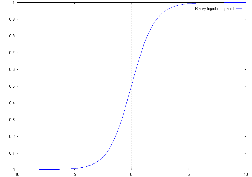
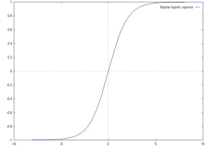
Every node can have its own activation function, however generally only two activation functions are used in a particular network. The input layer and sometimes the output layer use the identity function. When the output layer does not use the identity function, it will probably use the same activation function as the hidden layers. The hidden layers use any differentiable, non-linear function. Why? If the hidden layers use a linear activation function, their ability to produce categories that are not linearly separable is lost. If the function is not differentiable, you cannot apply the training algorithm used for back propagation networks. The most common activation functions used for the hidden layers and output layers are the binary or bipolar logistic sigmoid. To gain an understanding of what these functions do, it is convenient to look at their graphs. The graphs for both functions are as follows.

![]()
![]()
As you can see both functions meet the criteria given for the activation functions. They are differentiable and non-linear.
Now that the architecture for back propagation networks is out of the way, we can take a look at the training algorithm for them. For the purposes of this discussion, we will assume the network has only one hidden layer. The argument that follows does not change if multiple hidden layers are used, but the notation gets very ugly and confusing. If you recall the training algorithm for back propagation networks is based on the training rule for the adaline, the delta rule. The modified training rule, the generalized delta rule, uses the same concept to train a neural network. The goal is to minimize the overall error on the network by finding an optimum set of weights. Once again, if we wish to minimize the error, a mathematical expression for the error is needed. If the network has m output nodes,
![]()
This function should look very familiar. It is almost exactly the same as the error function used for the delta rule. In fact, the only difference is that the difference between the desired output, tj, and actual output, yj, is used instead of the difference between the desired output and the net input to the output node, y_inj. Recall that we stated the activation function for an output node must be the identity function or some other differentiable function. Because of this restriction, we are not forced to use the net input to the output node in our error function.
Next, expressions for the net input to an output node and
hidden node are needed to continue the discussion of the
generalized delta rule. The net input to any node is the weighted
sum of its input signals. Hence the expression, ![]() can be used to calculate
the net input for the output node J. Because we have an extra
layer in this network, the hidden layer, some new symbols are
used. In the above expression, p represents the number of hidden
nodes, and zk represents the activation for hidden node k. The
other symbols should look familiar. The net input for the hidden
node K is calculated using the expression,
can be used to calculate
the net input for the output node J. Because we have an extra
layer in this network, the hidden layer, some new symbols are
used. In the above expression, p represents the number of hidden
nodes, and zk represents the activation for hidden node k. The
other symbols should look familiar. The net input for the hidden
node K is calculated using the expression, ![]() where viK is the weight from input node
i to hidden node K.
where viK is the weight from input node
i to hidden node K.
Just as in the derivation for the delta rule, we proceed by taking the partial derivative of the error with respect to each one of the weights between the hidden and output nodes. The sign of the partial derivative tells us in which direction to change the weights if we wish to increase the error. Therefore, we will multiply the partial derivative by negative one to find the direction in which the error decreases. For convenience in the calculations, we will multiply the error function by one half before differentiating. This has no effect on the sign of the derivative and thus does not effect our derivation of the generalized delta rule. In the following derivation, the function f(x) represents the activation function on the output node.
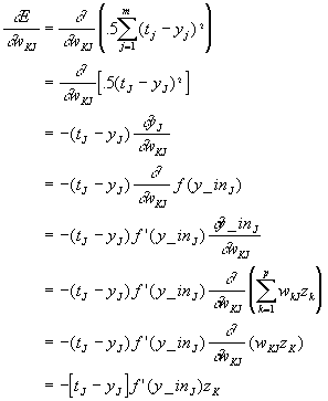
It is convenient to define d J:
![]()
Using the above expressions, we can calculate the weight changes for the weights between the hidden and output nodes. Once again, a learning rate constant is introduced to control the speed of learning.

Now that the weight change algorithm is known for the weights between the hidden and output layers, a weight change algorithm is needed for the weights between the input and hidden layers. The same process as above will be used to find this algorithm. However instead of differentiating with respect to the weights between the hidden and output layers, we will differentiate with respect to the weights between the input and hidden layers. In the following derivation, the function g(x) is the activation function for the hidden nodes.
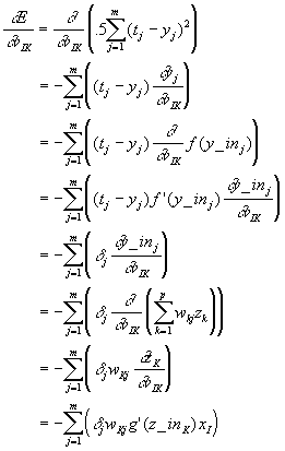
It is once again convenient to define d K:
![]()
We now can calculate the weight changes from the input to the hidden layers.
![]()
Don’t worry, the math is done. We have derived the generalized delta rule. The weight change rules given in figure 19 and 21, together form the generalized delta rule. It may be difficult to see, but if you examine the expression for d K you should be able to see that the error from the output nodes, d J , is being sent backwards, back propagated, along the connections to the hidden nodes. The error is then passed through the derivative of the activation function. So basically the error was sent backwards through the network to the hidden layer(s) and thus the weights between the input and hidden layers could be adjusted.
Using the generalized delta rule to train a back propagation network is identical to using the delta rule to train the adaline. So, instead of repeating the entire process, you can refer to the section on adalines to refresh your memory on how to apply the generalized delta rule.
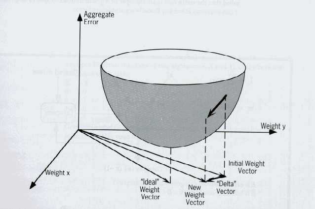
The training algorithm derived above is the most common form of the generalized delta rule, however certain researchers have made various improvements to the rule. One change, that dramatically improves the learning process, is the addition of a momentum. If you perceive the error function as a three dimensional surface, with the weights as the x and y axis’s and the error as the z axis, placing a marble anywhere on the surface will represent the initial weights of the neural network. Training the neural network using the generalized delta rule is then akin to letting the marble go and having it settle in a valley of the surface. The location of this valley, a local minimum for the error, represents the final weights produced by the training algorithm. If our comparison is to be perfect, we must move this entire system to a place where the laws of physics cease to exist. More specifically, the ball should have no momentum. It should not gain speed as it descends down the hill to the valley, instead it should have a constant speed.
However, if we introduce a momentum term to the generalized delta rule, we can take the system back into the normal universe. The ball, with its momentum returned, now approaches the valley quicker than it did when its momentum was removed. This is exactly what occurs when a momentum term is introduced into the generalized delta rule. Because of the significantly improved performance, the back propagation network is rarely used with this momentum term.
![]()
Home Page ![]() Introduction
Introduction ![]() Biological Neural
Networks
Biological Neural
Networks ![]() McCulloch-Pitts Neuron
McCulloch-Pitts Neuron
Perceptron ![]() Adaline
Adaline ![]() Back Propagation
network
Back Propagation
network
References ![]() Research Paper
Research Paper ![]() Glossary
Glossary
![]() Beware: This
page is always under construction
Beware: This
page is always under construction
![]() Geocities
Geocities
![]() Geocities
Research Triangle
Geocities
Research Triangle